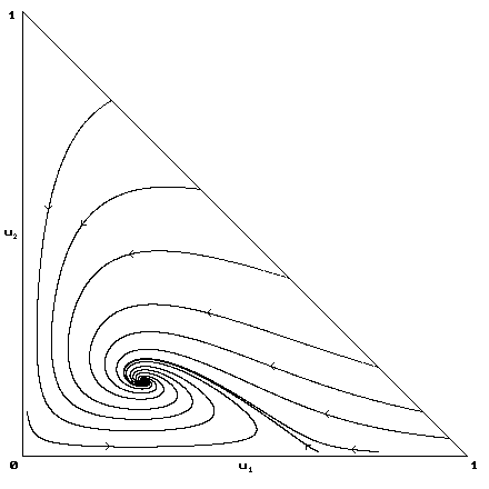
Here the possible states are 0 = vacant, 1 = prey, 2 = predator. Letting f[i] be the fraction of neighbors in state i we can formulate the dynamics as follows:
1's behave like a contact process, dying at a constant rate d[1] and being born at vacant sites at rate b[1]f[1].
2's die at a rate d[2] + cf[2], with the second term representing competition between predators. 2's are born at sites occupied by 1's at at rate b[2] times the fraction of neighbors in state 2.
Finally, there is stirring at rate nu: for each pair of neighboring sites x and y we exchange the values at x and at y at rate nu.
Prey turning into predators may sound ludicrous but (i) this transition encodes the fact that the predator population will tend to decrease when prey are scarce, and (ii) the resulting mean field equation is a standard predator prey ODE:

For example, when b[1] = 3, b[2] = 4, d[1] = 1, d[2] = 1, and c = 0.5, the ODE looks like:

Solving two equations in two unknowns we see that there is a fixed point at

This point has both components positive when

The first condition says that prey are viable in the absence of predators. To see the reason for the second condition note that if 1's are in equilibrium and the density of 2's is small then the left-hand side is the birth rate (per occupied site) while the right-hand side is the death rate, so this guarantees that the density of 2's will increase when it is small. In words, the 2's can invade the 1's in equilibrium.
Durrett (1993) used the fact that rapid stirring limits of particle systems are reaction diffusion equations to show:
Theorem. If b[1] > d[1] and b[2] (b[1] - d[1])/b[1] > d[2]. then when the stirring rate nu is large the particle system has a stationary distribution in which the density of prey and predators are close to that of the fixed point of the ODE.
Using results of Durrett and Neuhauser (1994) it is fairly straightforward to show the converse
Math Exercise. Show that if b[1] > d[1] but we reverse the second inequality, b[2] (b[1] - d[1])/b[1] < d[2], then 2's die out when the stirring rate nu is large.
s3 Exercise. Set b[1] = 3.0, d[1] = 1, b[2] = 4.0, d[2] = 1.0, c = 0.5, and the fraction of stirring steps = 0.5. (These are the model defaults and the values for the ODE pictured above.) The simulation settles into an equilibrium in which about 20% of the sites are occupied by predators and 30% by prey, though on the default 120 x 120 grid there are small oscillations in the density. The picture shows some rather obvious correlations between neighboring sites, so it should not be surprising that there is some difference between the equilibrium frequencies in the spatial model and those predicted by the mean field ODE: 16.9% predators, 27.1% prey.
s3 Footnote. To increase the effect of single stirring steps we exchange the value at x with a site y chosen at random from the square of radius 3 centered at x.
Durrett, R. (1993) Predator-prey systems. Pages 37--58 in Asymptotic problems in probability theory: stochastic models and diffusions on fractals. Edited by K.D. Elworthy and N. Ikeda. Pitman Research Notes 83, Longman Scientific, Essex, England
Durrett, R. and Neuhauser, C. (1994) Particle systems and reaction diffusion equations. Ann. Probab. 22, 289-333