Some strains of E. coli produce a substance called colicin that kills competing strains. The producing strains are immune to the action of this chemical but reproduce at a reduced rate because some of their metabolic energy is devoted to its production. To study this situation we will use a model with states 0 = vacant, 1 = colicin producer, 2 = colicin sensitive E. coli. Letting f[i] = the fraction of neighbors in state i we can formulate the dynamics as:
1's die at a constant rate d and are born at vacant sites at rate b[1]f[1].
2's die at rate d + cf[1] and are born at vacant sites at rate b[2]f[2].
In words each species is a contact process but 2's have an extra death rate due to production of colicin by neighboring 1's.
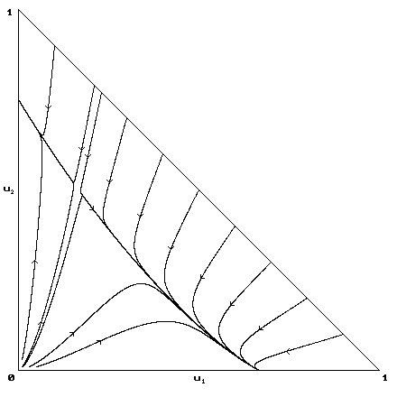
To guess what will happen in this model we look at the mean field ODE. Here u[0] = 1 - u[1] - u[2], so the system is two dimensional.

Letting v[i] = (b[i]-d[i])/b[i] there are boundary equilibria at (v[1],0) and (0,v[2]). There will be an interior equilibrium if

However, the interior equilibrium is always a saddle point, while the two boundary equilibria are locally attracting. For example when b[1] = 3, d[1] = 1, b[2] = 4, d[2] = 1, and c = 2:

The local attractivity of the boundary equilibria are locally attracting implies that if the density of colicin producing bacteria is small, it will decrease. This situation is sometimes called disruptive frequency dependent selection since colicin production is only favored when it is fairly common.
In contrast in a spatial model there is (for generic parameter values) one stronger type that takes over the system when it starts with a positive density. To identify the stronger type we start the system with all 1's on the left half and all 2's on the right half. If the front between the two types moves to the right (resp. left) at a positive speed, then 1's (resp. 2's) are stronger. In the nongeneric case in which the front speed is 0, there is no stronger type.
The conclusions in the last paragraph have not been proved but they are easy to demonstrate by simulation.
s3 Exercises. For all of these set b[1] = 3.0 and b[2] = 3.5.
1. Choose the random initial condition. When c = 1.0, 1's win but when c = 0.5, 2's win.
2. Set c = 2.0, and choose the product measure initial condition with 1's having density 0.5 and 2's having density 0.01. Note that 2's form blobs that grow linearly and take over the system.
3. Set c = 2.0 and choose the half-half initial condition. Check that that the 1 region expands but be prepared to wait for a long time to see this.
Chao, L. and Levin, B.R. (1981) Structured habitats and the evolution of anti-competitor toxins in bacteria. Proc. Nat. Acad. Sci. 78, 6324--6328
Levin, B.R. (1988) Frequency dependent selection in bacterial populations. Phil. Trans. Roy. Soc. B. 319, 459-472
Frank, S.A. (1994) Spatial polymorphism of bacteriocins and other allelopathic traits. Evolutionary Ecology. 5, 193--217
Durrett, R. and Levin, S. (1997) Allelopathy in spatially distributed populations. J. Theor. Biol., to appear