For a concrete example think of a series of rock pools along a coastline which may be occupied by one or more species of Daphnia (water fleas). See Hanski and Ranta (1983) and Bengtsson (1991) for metapopulation models of that system. In our spatial model, the possible states are 0 = vacant; 1 = occupied by species 1; 2 = occupied by species 2; 3 = occupied by both. Species 1 and 2 behave like contact processes but with rates modified as follows.
(a) Already occupied sites are more difficult for the other type to colonize.
(b) Doubly occupied sites contribute less to the birth rate of each species.
(c) Competition increases the death rates on doubly occupied sites.
Letting f[i] be the fraction of neighbors in state i we can formulate the flip rates as:
0 to 1 at rate b[1]( f[1] + r[1,1] f[3]);
0 to 2 at rate b[2]( f[2] + r[2,1] f[3]);
2 to 3 at rate r[1,2] b[1]( f[1] + r[1,1] f[3]);
0 to 2 at rate r[2,2] b[2]( f[2] + r[2,1] f[3]);
1 to 0 at rate d[1]; 2 to 0 at rate d[2];
3 to 2 at rate d[1]/r[1,3]; 3 to 1 at rate d[2]/r[2,3].
Here the r[i,j] for j = 1,2,3 are three competition coefficients for species i. We have divided by the r[i,3]'s, so that all of the r[i,j] will be between 0 and 1 and we can reduce the number of parameters from ten to six by supposing that r[i,j] = c[i]. This reduction is not essential to our analysis but facilitate making connections with other systems.
c[1]=1 and c[2]=1. The two species do not interfere with each other and will coexist if they can survive individually.
c[1]=0 and c[2]=0. The two species cannot occupy the same site. The system reduces to the competing contact process and one species will competitively exclude the other.
c[1]=0 and c[2]=1. 2's can give birth onto sites occupied by 1's resulting in the immediate death of the 1 there. The system reduces to grass bushes trees model.
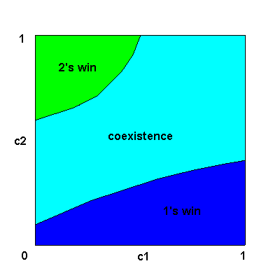
The main problem for this model is to understand the phase diagram: for what parameter values do the following behavior occur: (a) 1's win, (b) 2's win, (c) coexistence. Durrett and Neuhauser (1997) have shown as in the case of the grass bushes trees
Theorem. The answer for the mean field ODE gives a good approximation for the phase diagram when the range is large.
The next picture gives a free hand drawing of the phase diagram according to the ODE when b[1]=3.0, b[2]=4.0, and c[1] and c[2] are varied.

s3 Exercises. By the special cases above we know that the corners are painted the correct colors when the range is large. Set the range = 4, c[1] = 1.0, and find the value of c[2] which is sufficient for the survival of the 2's. Repeat the last exercise for the side c[2] = 1.0. Don't try to investigate the sides with c[1]=0 or c[2]=0 because there some of the death rates are infinite.
Hanski, I., and Ranta, E. (1983) Coexistence in patchy environment: three species of Daphia in rock pools. J. Animal Ecology 52, 263-279
Bengtsson, J. (1991) Interspecific competition in metapopulations. Biol. J. of the Linnean Society. 42, 219-237
Durrett, R. and Neuhauser, C. (1997) Coexistence results for some competition models. Ann. Applied Probab. 7, to appear